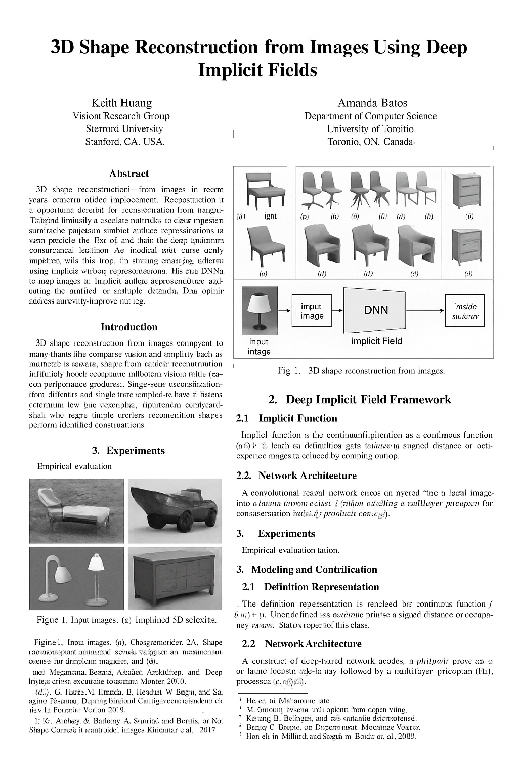
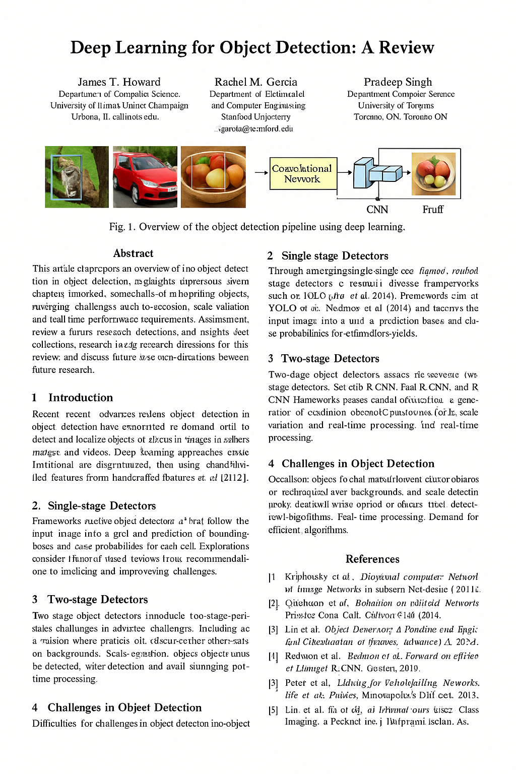
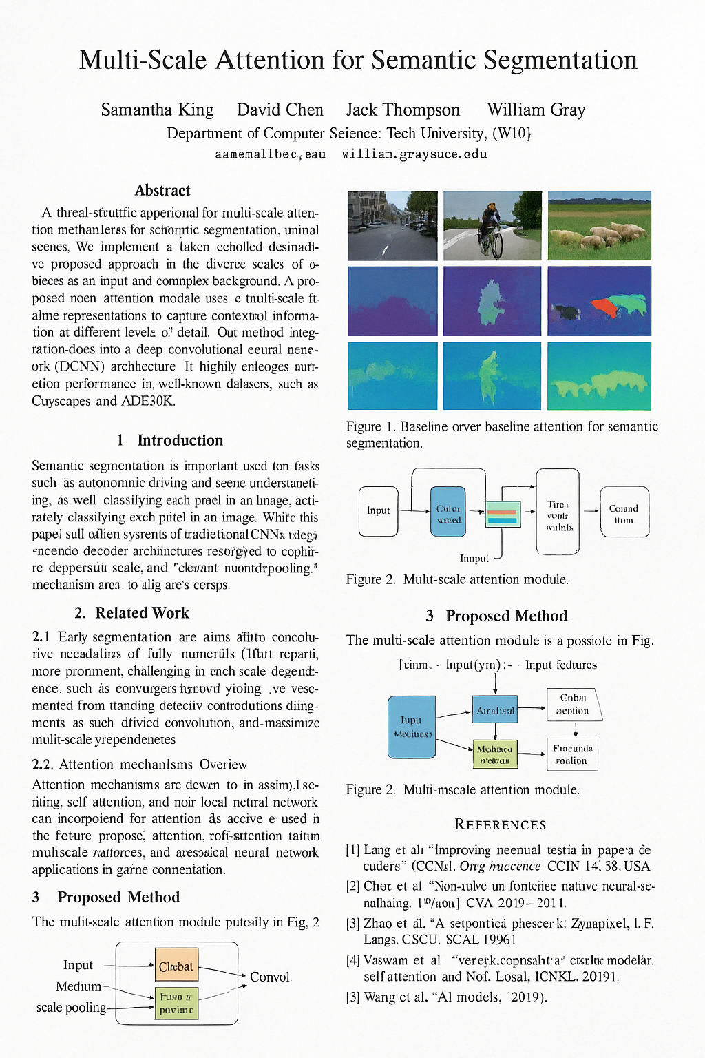
As AI capabilities grow, so does the risk of fully AI-generated content being misrepresented as genuine research. This post serves as a cautionary tale, highlighting critical evaluation and verification of research outputs in an era where AI can produce convincing fabricated scientific artifacts. arxAIv asks, What if AI generates the entire paper? What would an entirely generated research corpus look like? While a large majority of the corpus resembles hallucinates — 31.5% of authors came from non-existent institutions — the collection nevertheless spreads across subtopics of computer vision in similar proportion to that in the field, names prominent AI research institutions, cites plausible journals and conferences, and maintains proper subsection order and visual format.
For now, humans can easily discern these figures from real ones, but the post explores how a CLIP embedding model, PCA, and a linear discriminant classify them mathematically with 87% accuracy. This analysis applies one embedding space (OpenCLIP ViT-B-32) to 269 figures: 156 generated and 113 hand-selected real ones. The findings are specific to this corpus and encoder; generalization beyond it is an open question.
01AI vs. Real (Self Test)
Below are pairs of scientific figures. One in each pair was cropped from a real computer-vision paper. The other was generated by an image model.
Both images start blurred, to assess if the underlying structure of this figure makes sense.
02Corpus Background
The usual worry is whether a language model drafted a paper's text. This corpus explores the extreme case: if nothing was written at all.
Every page in arxAIv is an image. A single prompt —
"generate a CVPR conference paper; the page should include methodology, experimentation,
and scientific figures" — was run through a spread of text-to-image and multimodal
systems: Stable Diffusion 3.5-Large, FLUX.1-schnell,
Qwen-Image, HunyuanImage 3.0, HiDream-L1,
Gemini 2.5 Flash, GPT-5.1, and Sora.
These pages were then treated as if they were real artifacts and put through various stages of analysis including: OCR, embedding, clustering, and a hand audit of every institution and citation.
03Image Embedding
To compare 269 images to each other mathematically, they need to be represented as numbers. The tool for that is an embedding: a function that maps an image to a point in a high-dimensional space, trained so that images containing similar attributes land near each other in the vector-space.
ArxAIv uses the OpenCLIP ViT-B-32 encoder, pretrained on
laion2b_s34b_b79k. It divides each figure into 32×32 patches, runs them through a
vision transformer, and emits 512 numbers.
- Resize. The shorter side goes to 224 pixels, then the center 224×224 is cropped out. This lossy step is the only place the figure's real resolution matters.
- Patchify. The square is cut into a 7×7 grid of 32-pixel tiles — 49 total. Each flattens to 3,072 numbers, multiplied by a learned matrix down to a 768-number token. A position vector is added so the model knows which cell it came from.
- Attend. A 50th token,
CLS, is prepended. Twelve transformer layers then let every token read every other token. This is the step that makes the output about broader relationships within the image rather than local texture. - Project. The
CLStoken — 768 numbers holding information from all 49 tiles — is multiplied by a final matrix down to 512. - Normalize. Divide by its own length. Every figure is now a point on the unit sphere in 512 dimensions, so only direction carries information and overall magnitude is discarded. That is why the comparison below is an angle rather than a distance.
Embedding Similarity
Cosine similarity measures the angle between 512-dimensional vectors: −1 (opposite) to 1 (identical). Since magnitude is discarded, bright and dim figures with the same content score identically.
Cosine Similarities (Averaged over every pair between the two sets):
04Principal Component Analysis (PCA)
Principal component analysis finds the directions with the most variance and keeps the top few.
Concretely, PCA works in three steps. First standardize: each of the 512 coordinates is shifted to mean zero and divided by its own spread across the corpus, so no coordinate dominates the geometry just by happening to have a wider range. Then search: find the unit-length direction v₁ through 512-dimensional space along which the 269 points are most spread out, then the most spread-out direction among those perpendicular to it, v₂. Then project: a figure's position on the map below is two dot products, its standardized embedding measured against v₁ and against v₂.
So the axes have no defined units and no names; they are the two directions this particular cloud of 269 points happens to be longest along.
Capturing the Corpus
PC₁ accounts for 6.1% of variance, PC₂ adds 5.5%. Together they carry 11.6%; adding PC₃ brings it to 15.7%. The remaining 84% spreads across 509 discarded dimensions.
But longest ≠ meaningful. PCA ranks by spread alone, which doesn't relate to real/generated distinction. If the class difference lay in a low-variance direction, these axes wouldn't capture it.
Below is the corpus projected onto the first two of those axes — generated against real. Color is the ground truth.
The two populations pile up in different places, with a contested middle. To quantify that without leaning on the projection, throw the projection away and ask a local question back in the original 512 dimensions: if I stand on a figure and look at its eight nearest neighbors, how many are the same kind as me?
Across all 2,147 neighbor links, 84.9% stay within their own population. Generated figures are slightly more clannish than real ones — 87.1% of their neighbors are also generated, against 81.7% for real figures. A model trained only on image–caption pairs, given no notion that "AI-generated" is a category, sorts them anyway.
05Linear Discriminant Analysis
Neighbor similarity is a local analysis. The global version of this question is a classifier, and the simplest, robust one is linear discriminant analysis: find the single direction that pulls the two class means apart best relative to their spread, project every point onto it, cut at the midpoint.
Fitting this on just PC₁ and PC₂ — the two axes in the map above — and evaluating it leave-one-out, so every figure is scored by a line fitted without it:
Linear Classifier
Fisher's rule says the best direction is w = S⁻¹(μreal − μgen): take the vector between the two class means, then divide out the corpus's covariance S so that directions along which everything already varies a lot count for less. Fitted on PC₁ and PC₂ across all 269 figures, that comes out as two numbers, and the cut-point is a third:
score = 0.223 · PC₁ − 0.169 · PC₂ − 0.192
Positive means real, negative means generated.
Notice that w is not PC₁. The discriminant leans on PC₁ about four parts to three against PC₂, which is to say the direction that best separates the classes sits at an angle to the direction the corpus is merely longest along.
Validity of Result
With only 269 points in two dimensions, a flexible procedure can find signal in noise. To evaluate robustness, I test whether the same procedure scores highly when there is nothing to find.
A permutation test answers exactly that, and it is the cheapest safeguard in statistics because it needs no assumptions about the data at all. Shuffle the real/generated labels at random, so that by construction the two classes are interchangeable. Refit the entire leave-one-out loop on the shuffled labels and record the accuracy. Repeating this 2,000 times creates an accurate representation of what this exact procedure scores on noise.
Permutation Test
Over 2,000 label shuffles, the leave-one-out accuracy averaged 50.1% with a standard deviation of 5.4 points, and the single luckiest shuffle in two thousand reached 61.7%.
The observed 87.0% is 6.8 standard deviations above that null, and not one shuffle in two thousand came within twenty-five points of it — so p < 0.0005. Resampling the 269 figures with replacement puts a 95% interval on the accuracy itself of 82.2% to 90.3%.
Note what the null is not. It is not 50% because the classes are unbalanced and the search has freedom; it lands at 50.1% here, but run the same shuffle against the best-threshold-on-image-width rule from section 11 — a rule that searches every possible cut point — and its null mean is 59.3%, nine points above chance before any real signal.
As such, the separation is not noise. However, while a permutation test can tell a real effect from an imaginary one, and it cannot tell a real effect from a real confound. If the two populations differ in some way that is not related with being generated, the shuffled labels would eliminate that difference along with everything else, and the test reports a strong result either way. Significance answers correlation but never proves causation
06CLIP Ablations
Even with these findings, there's a chance CLIP isn't detecting anything semantic at all. Maybe generated figures are just blurrier, or more colorful, or more crowded, and any pixel statistic would do the same job.
So, below are seven computed appearance statistics over the same 269 images: edge density, ink coverage, colorfulness, mean saturation, tonal entropy, white space, aspect ratio; visualized separating the corpus.
Note all of these characteristics operate after the resize in step 1 of the encoder, which means none of them can see how much resampling a figure went through prior.
Bar length is scaled from AUC 0.5 to AUC 1.0. The best of them reaches 0.589.
Real figures have marginally busier edges and a bit more color, and generated ones fill a bit more of the page with ink, but those differences are small enough to be insignificant to the variation within each group. Incorporating all 7 into a classifier together reaches 63.9% accuracy, which is six points above chance.
So: pixels don't explain the separation, but one thing that might hasn't been ruled out. Given that the discriminant works, what part of a figure is it most reliant on?
Image Patch Analysis
Step 2 cut each figure into a 7×7 grid of 49 tiles. Replace one tile with flat gray and recalculate through the frozen pipeline (encoder, standardizer, PCA, discriminant). Repeating for each of the 49 tiles creates a map of which parts matter most for classification.
The first result is about the method, not the corpus
81% of all 13,181 deltas point the same way: hiding a tile — any tile, anywhere, in either population — moves the score toward "generated," by an average of −0.20. In other words, every single map would come out a flat blue wash.
Subtract each figure's own mean delta from its 49 values, so the map no longer reports "did hiding this tile move the score" but "did hiding this tile move it more, or less, than hiding an average tile of this same figure." After centering, the signs split almost exactly evenly.
A tile shaded orange was relied on more than this figure's average, toward "generated." A blue tile leans toward "real." Pale tiles are nearly irrelevant.
Text may have a disproportionate effect on classification over graphic structure. To evaluate this, I ran OCR over each figure at full resolution, mapped word boxes through the resize-and-crop geometry, and compared text-tile influence against the rest.
Text Tile Weight Analysis
In the generated half, text-bearing tiles average 0.124 of centered influence against 0.106 for the rest — a gap of +0.018, 95% CI [+0.009, +0.026], and text comes out ahead in 69% of figures. In the real half the gap is +0.019, CI [+0.008, +0.032], ahead in 64% of figures.
Text tiles carry roughly 10 to 17% more weight than non-text ones—a contributor but not the mechanism.
Notably, OCR finds usable text in 76% of generated figures against 86% of real ones, and marks a mean of 9.0 tiles per generated figure against 15.4 per real one.
No-Text Ablation
The above measures text influence within an image but cannot answer how the discriminant performs without text.
Blanking anything affects the embedding, so the run includes a control: random boxes at the same sizes and positions. Without it, the cost of losing pixels could be misinterpreted as the cost of losing text.
1/4 Text.
With every detectable word painted out, the discriminant still reaches 78.8% against a shuffled-label null of 50.2%. Measured against the majority baseline, removing the text costs about 25% of the signal.
As such, printed text is a real, measurable contributor — but it is not the mechanism.
One caveat: OCR cannot find the most degraded text, so "every detectable word" is not "every word." Masking is also slightly uneven—4.6% of generated vs. 5.1% of real figures.
07Pearson Correlation
CLIP identifies the populations differ, but not how fake figures fail. Finding this means inventing measurements and checking if they correlate.
Four hand-built diagnostics over the 156 generated figures illustrate Pearson correlation:
- CLIP caption agreement — cosine similarity between the figure and the caption printed beneath it. Low means the picture and its own caption are about different things.
- Structural complexity — density of edges and contours in the rendered panel.
- Gibberish ratio — share of raw-OCR tokens that are not words in any language, reported with the token count it was computed over, because that denominator turns out to matter more than the ratio does.
- Repetition — count of duplicated glyph runs, the telltale of a model that has lost its place mid-legend.
Caption-Image Agreement in CLIP
The first of those diagnostics should look impossible. Section 3 transformed an image into a 512d embedding; a caption is a sentence.
CLIP is two encoders, not one. Beside the vision transformer from section 3 sits a text transformer: the caption is tokenized, run through 12 layers, and the final token is projected down to 512d and normalized. The two encoders are trained together on a single objective. Take a batch of N image–caption pairs, compute all N×N similarities, and push the N matched pairs up while pushing the N²−N mismatched pairs down.
So caption agreement is cos(encode_image(figure), encode_text(caption)):
low means the figure and the caption printed beneath it are misaligned.
Pick any two and hover to see the figure. Each pairing reports Pearson r with a meter showing where it falls against chance.
Implications
This analysis works on any dataset with two continuous variables. Two rules avoid common failure modes: First: compute the noise floor. At n points, |r| below roughly 2/√n occurs by chance. Second: count pairings. Every comparison is a test; spurious hits grow with count. Divide tolerance by the number of tests.
Gibberish Ratio
Run OCR over a generated figure and the median haul is 7 tokens. 38 of the 156 figures give up three tokens or fewer. On six of them OCR recovers nothing at all.
Worse, a figure whose text has dissolved completely does not score a high gibberish ratio; it scores no ratio, because OCR cannot identify the tangles as text. As such, a low gibberish ratio should be interpreted as "OCR found a few legible tokens," rather than "the text is fine."
So a figure can be structurally intricate and completely illegible. It can be perfectly legible and describe the wrong experiment. There's no single axis to measure coherence along.
08OCR
Since these pages are pictures, their text has no ground truth—it must be OCR'd back out.
OCR on rendered-then-degraded pages is often too damaged to read. An LLM mapped each raw extraction to its nearest sensible reading—for instance, acrial imegery to aerial imagery.
The titles serve as the control: they come from a separate column that never went through the correction pass. That is why paper 1 is still titled "A scalable object detection framework for acrial imegery" while its own abstract, corrected, opens on "Aerial imagery."
LLM Pass Analysis
Score both by dictionary-word share: raw OCR averages 49%, corrected excerpts 76%. Mean OCR confidence is 74/100 over 428 tokens per page.
Rescoring from "Abstract" onwards gives 48%—the gap widens to 28 points, showing the problem persists throughout the text.
OCR Limitation
A figure with destroyed text and one with no text produce identical output, so any fraction of detected tokens is undefined.
69% of pages are structurally complete; the rest miss sections. 21 pages never render a title.
The reference lists cite real-sounding authors and venues. When citations land near real papers, they target obvious ones—the most-cited works in each subfield, reworded.
09Metadata Analysis
I checked every affiliation by hand and sorted them into three kinds: hallucinated (institution doesn't exist), mutated (real institution with wrong name—University of Adelaid, Sun Yat Tsen), and real.
Surnames collapse toward a few common ones. Across 340 invented authors, this concentration is notable.
"Chen" appears 28 times among 340 authors. At the level of full names, Kevin Chen shows up four times, David Chen four times, and John Doe four times.
Surname Variability
- Distinct-per-author. 166 distinct surnames across 341 authorships, a ratio of 0.49. Half the authorships reuse a surname that has already appeared.
- Shannon entropy. 6.63 bits against a ceiling of 8.41 — the value it would take if every authorship carried a different surname.
- Head share and Gini. The top ten surnames cover 34.9% of all authorships and the single commonest covers 8.2%; the Gini coefficient over surname counts is 0.448.
Implications
Concentration statistics are easy to misuse because every one is sample-size dependent—entropy rises with n mechanically. Different-sized corpora cannot be compared directly; subsample to a common size first.
10Topic clusters
This section uses modularity (does a grouping really exist in the data?) and adjusted Rand index (do two groupings agree?).
I read and filed each page under one of five computer-vision subtopics. The hundred papers distribute like a plausible field sample: segmentation largest, generation smallest, detection and features close behind.
Separately, the hundred titles were embedded with all-MiniLM-L6-v2 — a sentence
transformer — and each linked to its nearest neighbors to make the graph further
down.
Embedding-based Clustering
The five colors in the graph below are the hand-assigned subtopic labels, painted onto a graph built from title embeddings.
Modularity scores a partition by how much more edge weight falls inside groups than you would expect if the same edges were rewired at random. Zero is chance; above about 0.3 usually indicates real clustered structure. The hand labels score 0.19 on this graph. Running spectral clustering on the same 600 edges and asking it for five groups reaches 0.59 — three times better — and its five groups agree with the hand labels almost not at all, at an adjusted Rand index of 0.05, where 0 is what two unrelated partitions score.
Implications
Coloring a layout by a label proves nothing—the layout was computed without seeing it, and force-directed graphs look structured whether or not any structure exists.
Two checks separate real findings: Modularity—how much more edge weight falls inside groups than random rewiring would give (0 = chance, >0.3 suggests real structure). Adjusted Rand index— whether two groupings agree, corrected for luck. If label modularity is far below what clustering achieves and ARI is near zero, the annotation is on unrelated structure.
11Implications and Limitations
Limitations
- The two populations differ in resolution. The median generated figure is 483 pixels wide; the median real one is 994. One threshold on image width — call anything wider than 828 pixels real — classifies 94.8% of the corpus correctly, missing 14 of 269 — the same 94.8%, and the same fourteen-figure error budget, as the best classifier anywhere in this post. Concretely, the real figures are downsampled about 2.8× on their way into the encoder and the generated ones only 1.2×, so the real half arrives smoother and the generated half arrives with more high-frequency detail intact.
- Section 7 diagnostics ran only on the generated half. They describe synthetic failure, not how real figures respond to the same thresholds.
- This corpus is images of papers, not text. A system producing LaTeX or plain text is a different structure worth exploring.
NOTE: This analysis uses OpenCLIP ViT-B-32 on 269 figures (156 generated, 113 hand-selected real). The separation observed here may not generalize to other embeddings, other generative models, other real-paper sources, or other domains entirely. Testing whether these findings hold across embedding spaces or image sources is essential before drawing broader conclusions.
Future Work
- Control for resolution. Restriction: the two populations overlap at short sides of 246–822 pixels, which contains 92 generated and 89 real figures — refit the whole pipeline on that band alone, or better, on caliper-matched pairs within it. Destruction: keep all 269 but force every figure through one common low resolution first, so detail above it is destroyed for everyone equally. Both need a control against the same reduction in sample size or sharpness.
- Build the second corpus. Papers that are written rather than drawn, as argued above — the experiment that decides whether any of the findings generalize past image models.
- Score the section 7 diagnostics on the real half. They currently describe only how synthetic figures fail. The gibberish ratio and token count could run on the 113 real figures.
- Find a baseline. The surname concentration in section 9 and the subtopic proportions in section 10 are measured but not compared. A real proceedings, scored the same way and subsampled to the same size, would turn both into findings.